 点击上方蓝字关注我们
微信公众号:OpenCV学堂
关注获取更多计算机视觉与深度学习知识
免费领学习资料+微信:OpenCVXueTang_Asst
介绍
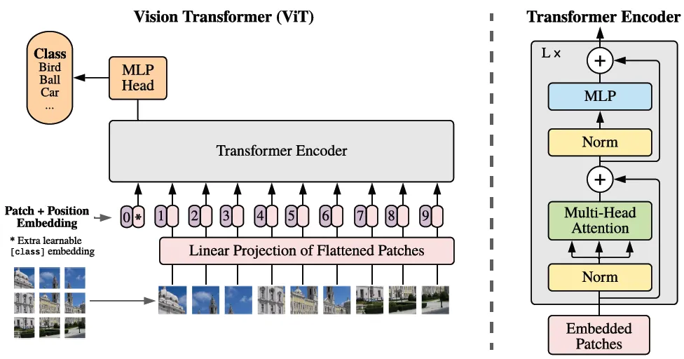
ViT的架构
代码实现
01
图像嵌入转换
class Embeddings(nn.Module):
def __init__(self, config):
super().__init__()
self.config = config
self.patch_embeddings = PatchEmbeddings(config)
# Create a learnable [CLS] token
# Similar to BERT, the [CLS] token is added to the beginning of the input sequence
# and is used to classify the entire sequence
self.cls_token = nn.Parameter(torch.randn(1, 1, config["hidden_size"]))
# Create position embeddings for the [CLS] token and the patch embeddings
# Add 1 to the sequence length for the [CLS] token
self.position_embeddings = \
nn.Parameter(torch.randn(1, self.patch_embeddings.num_patches + 1, config["hidden_size"]))
self.dropout = nn.Dropout(config["hidden_dropout_prob"])
def forward(self, x):
x = self.patch_embeddings(x)
batch_size, _, _ = x.size()
# Expand the [CLS] token to the batch size
# (1, 1, hidden_size) -> (batch_size, 1, hidden_size)
cls_tokens = self.cls_token.expand(batch_size, -1, -1)
# Concatenate the [CLS] token to the beginning of the input sequence
# This results in a sequence length of (num_patches + 1)
x = torch.cat((cls_tokens, x), dim=1)
x = x + self.position_embeddings
x = self.dropout(x)
return x
02
多头注意力
class AttentionHead(nn.Module):
"""
A single attention head.
This module is used in the MultiHeadAttention module.
"""
def __init__(self, hidden_size, attention_head_size, dropout, bias=True):
super().__init__()
self.hidden_size = hidden_size
self.attention_head_size = attention_head_size
# Create the query, key, and value projection layers
self.query = nn.Linear(hidden_size, attention_head_size, bias=bias)
self.key = nn.Linear(hidden_size, attention_head_size, bias=bias)
self.value = nn.Linear(hidden_size, attention_head_size, bias=bias)
self.dropout = nn.Dropout(dropout)
def forward(self, x):
# Project the input into query, key, and value
# The same input is used to generate the query, key, and value,
# so it's usually called self-attention.
# (batch_size, sequence_length, hidden_size) -> (batch_size, sequence_length, attention_head_size)
query = self.query(x)
key = self.key(x)
value = self.value(x)
# Calculate the attention scores
# softmax(Q*K.T/sqrt(head_size))*V
attention_scores = torch.matmul(query, key.transpose(-1, -2))
attention_scores = attention_scores / math.sqrt(self.attention_head_size)
attention_probs = nn.functional.softmax(attention_scores, dim=-1)
attention_probs = self.dropout(attention_probs)
# Calculate the attention output
attention_output = torch.matmul(attention_probs, value)
return (attention_output, attention_probs)
class MultiHeadAttention(nn.Module):"""Multi-head attention module.This module is used in the TransformerEncoder module."""def __init__(self, config):super().__init__()self.hidden_size = config["hidden_size"]self.num_attention_heads = config["num_attention_heads"]# The attention head size is the hidden size divided by the number of attention headsself.attention_head_size = self.hidden_size // self.num_attention_headsself.all_head_size = self.num_attention_heads * self.attention_head_size# Whether or not to use bias in the query, key, and value projection layersself.qkv_bias = config["qkv_bias"]# Create a list of attention headsself.heads = nn.ModuleList([])for _ in range(self.num_attention_heads):head = AttentionHead(self.hidden_size,self.attention_head_size,config["attention_probs_dropout_prob"],self.qkv_bias)self.heads.append(head)# Create a linear layer to project the attention output back to the hidden size# In most cases, all_head_size and hidden_size are the sameself.output_projection = nn.Linear(self.all_head_size, self.hidden_size)self.output_dropout = nn.Dropout(config["hidden_dropout_prob"])def forward(self, x, output_attentions=False):# Calculate the attention output for each attention headattention_outputs = [head(x) for head in self.heads]# Concatenate the attention outputs from each attention headattention_output = torch.cat([attention_output for attention_output, _ in attention_outputs], dim=-1)# Project the concatenated attention output back to the hidden sizeattention_output = self.output_projection(attention_output)attention_output = self.output_dropout(attention_output)# Return the attention output and the attention probabilities (optional)if not output_attentions:return (attention_output, None)else:attention_probs = torch.stack([attention_probs for _, attention_probs in attention_outputs], dim=1)return (attention_output, attention_probs)
03
编码器
class MLP(nn.Module):"""A multi-layer perceptron module."""def __init__(self, config):super().__init__()self.dense_1 = nn.Linear(config["hidden_size"], config["intermediate_size"])self.activation = NewGELUActivation()self.dense_2 = nn.Linear(config["intermediate_size"], config["hidden_size"])self.dropout = nn.Dropout(config["hidden_dropout_prob"])def forward(self, x):x = self.dense_1(x)x = self.activation(x)x = self.dense_2(x)x = self.dropout(x)return x
class Block(nn.Module):"""A single transformer block."""def __init__(self, config):super().__init__()self.attention = MultiHeadAttention(config)self.layernorm_1 = nn.LayerNorm(config["hidden_size"])self.mlp = MLP(config)self.layernorm_2 = nn.LayerNorm(config["hidden_size"])def forward(self, x, output_attentions=False):# Self-attentionattention_output, attention_probs = \self.attention(self.layernorm_1(x), output_attentions=output_attentions)# Skip connectionx = x + attention_output# Feed-forward networkmlp_output = self.mlp(self.layernorm_2(x))# Skip connectionx = x + mlp_output# Return the transformer block's output and the attention probabilities (optional)if not output_attentions:return (x, None)else:return (x, attention_probs)
class Encoder(nn.Module):"""The transformer encoder module."""def __init__(self, config):super().__init__()# Create a list of transformer blocksself.blocks = nn.ModuleList([])for _ in range(config["num_hidden_layers"]):block = Block(config)self.blocks.append(block)def forward(self, x, output_attentions=False):# Calculate the transformer block's output for each blockall_attentions = []for block in self.blocks:x, attention_probs = block(x, output_attentions=output_attentions)if output_attentions:all_attentions.append(attention_probs)# Return the encoder's output and the attention probabilities (optional)if not output_attentions:return (x, None)else:return (x, all_attentions)
04
ViT模型构建
class ViTForClassfication(nn.Module):
    """
    The ViT model for classification.
    """

    def __init__(self, config):
        super().__init__()
        self.config = config
        self.image_size = config["image_size"]
        self.hidden_size = config["hidden_size"]
        self.num_classes = config["num_classes"]
        # Create the embedding module
        self.embedding = Embeddings(config)
        # Create the transformer encoder module
        self.encoder = Encoder(config)
        # Create a linear layer to project the encoder's output to the number of classes
        self.classifier = nn.Linear(self.hidden_size, self.num_classes)
        # Initialize the weights
        self.apply(self._init_weights)

    def forward(self, x, output_attentions=False):
        # Calculate the embedding output
        embedding_output = self.embedding(x)
        # Calculate the encoder's output
        encoder_output, all_attentions = self.encoder(embedding_output, output_attentions=output_attentions)
        # Calculate the logits, take the [CLS] token's output as features for classification
        logits = self.classifier(encoder_output[:, 0])
        # Return the logits and the attention probabilities (optional)
        if not output_attentions:
            return (logits, None)
        else:
            return (logits, all_attentions)
参考
代码其实是我从github上面整理加工跟翻译得到的(个人认为非常的通俗易懂,有点pytorch基础都可以看懂学会),感兴趣的可以看这里:
https://github.com/lukemelas/PyTorch-Pretrained-ViT/blob/master/pytorch_pretrained_vit/transformer.pyhttps://tintn.github.io/Implementing-Vision-Transformer-from-Scratch/

原价:498
折扣:399
推荐阅读
OpenCV4.8+YOLOv8对象检测C++推理演示
ZXING+OpenCV打造开源条码检测应用
总结 | OpenCV4 Mat操作全接触
三行代码实现 TensorRT8.6 C++ 深度学习模型部署
实战 | YOLOv8+OpenCV 实现DM码定位检测与解析
对象检测边界框损失 – 从IOU到ProbIOU
YOLOv8 OBB实现自定义旋转对象检测
初学者必看 | 学习深度学习的五个误区
YOLOv8自定义数据集训练实现安全帽检测