用Matlab和Arduino构建4自由度机械臂（2）

一周前我转载了来自Circuit Cellar上的一篇技术含量非常高的文章：

用Matlab和Arduino构建4自由度机械臂（1）

今天续上第2节，同样也是英文的文章，转载在此，供学习技术的朋友阅读。原文来自Circuit Cellar官网，可以点击左下角的“阅读原文”直接阅读。

The Before and After Math

In Part 1, Raul discussed the general hardware and software aspects of his 4-DOF robotic arm project. In Part 2, he covers the topics related to the mathematical foundations of robotics. He then wraps up by talking about testing and debugging the robotic arm, and shares his thoughts regarding future improvements.

In Part 1 of this article (December 2019, Circuit Cellar 353), I presented the general hardware and software aspects of this project, including the electronics, the arm structure, the code for the embedded controller and relevant parts of the MATLAB code. I also talked about the PID controller implemented for joint 1 of the robotic arm, the serial command interface for receiving joint angle data in the embedded controller from the companion computer to control the robotic arm’s pose, how the MATLAB GUI interfaces with the application code, how to serially interface the companion computer with the embedded controller and how to plot the robotic arm’s pose in the MATLAB GUI.

In this second (and last) part, I’ll be discussing topics more related to the mathematical foundations of robotics, such as: configuration and task spaces, robot pose representation in three dimensions, homogeneous transformations, the Denavit-Hartenberg convention and forward and inverse kinematics. I will end by talking a bit about testing and debugging the robotic arm—and I’ll share my ideas about improvements.

CONFIGURATION AND TASK SPACES
The joint configuration of a robotic arm is the set of all joint angles that unequivocally describe their pose. It can be represented as a vector “q” containing all joint angles, as shown in Equation (1).

θ₁: joint 1 angle
θ₂: joint 2 angle
θ₃: joint 3 angle
θ₄: joint 4 angle

The configuration space of a robotic arm is the space of all possible joint configurations “q” that it can have. Their dimension is equal to the number of joints or degrees of freedom—in our case, four. The configuration space is constrained to a subset of all possible combinations of angles, because joints generally have physical limits, due to the arm structure design and motor rotation limits. Based on those limits, our robotic arm has constrained logical joint ranges, defined as follows:

θ₁: [-90,+90] (joint 1)
θ₂: [-25,+155] (joint 2)
θ₃: [-135,+45] (joint 3)
θ₄: [-90,+90] (joint 4)

For joints 2, 3 and 4, I’m using servo motors of 180 degrees, so in principle, these joints are physically constrained to a range between 0 and 180 degrees. However, for joint 1, I’m using a regular DC motor that can rotate in a range greater than the servo motors. I’m also constraining it to 180 degrees to uniform all ranges, while obtaining a reasonable work space for the robotic arm.

Now let’s explain how I defined those joint logical ranges. In the case of joint 2, for example, I took the 180 degrees of the servo motor’s physical range and defined a logical range of [-25, +155]. I did that after visually checking that’s the logical angle range that I wanted this joint to move in to obtain a reasonable work space. Then I did the same with the rest of the joints. Whenever the physical and logical ranges don’t coincide, there must be a conversion mapping between them. Figure 1 shows that’s the case for joints 2, 3 and 4.

FIGURE 1
Joint angle conversion mappings

ANGLE CONVERSIONS
When the embedded controller receives angles for these joints from the companion computer, it must convert the angles from their logical ranges (which are used in the companion computer for all operations, including kinematics calculations) to their corresponding physical ranges, before applying them to the motors. For instance, when joint 2 is at +155 degrees, that means its servo motor must be at 0 degrees. When it’s at -25 degrees, the servo motor must be physically at 180 degrees, and so on for all angles in between.

Aside from the fact that some joints must have specific range conversions, you can see in Figure 2 that although servo motors 2 and 3 are mounted in the same orientation, their physical ranges are reversed with respect to each other ([180, 0] vs. [0, 180]) in the conversion mapping. This is because when joint 2 rotates positively around its “z” axis (more on coordinate frames later), its servo motor goes toward zero physical degrees. But with joint 3 the opposite is true. You should check the orientation for each servo motor according your arm’s particular design, which, in turn, will define the orientation of their physical ranges in the conversion mapping (shown in Figure 1).

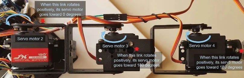
FIGURE 2
Robotic arm servo motor orientation

The Arduino “map” C language function allows an easy conversion of a value between two different ranges. For example the code line ang_conv = map(servo2_target_angle, SERVO2_INF_LIMIT, SERVO2_SUP_LIMIT, 180, 0) will perform the conversion for joint 2 shown in Figure 1. If, for any reason, your particular conversion mappings are different from the ones outlined in Figure 1, you should change all relevant “map” code lines in the embedded controller’s code to suit yours.

Figure 3 shows the pose of the robotic arm with all joints at zero logical degrees. This is also important to consider when mounting the motors in the mechanical structure. That’s because by following the Denavit-Hartenberg convention (which I’ll be discussing in more detail later) the zero-degree line of each motor must coincide with the “x” axis of its assigned coordinate frame. For example, applying the conversion mapping, zero logical degrees for joint 2 corresponds with 155 degrees of its servo motor. To mount joint 2 properly, we must put its servo motor at 155 degrees first, and then mount its link horizontally (Figure 3).

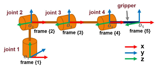
FIGURE 3
Robotic arm coordinate frame assignments

Finally, let’s quickly define “Task Space.” The Task Space of a robotic arm is defined as the set of all possible end effector poses. Their dimension is equal to the number of parameters used to describe the pose. In the case of our robotic arm, for simplicity I’m using a pose in three dimensions (x, y, z) without specifying orientation angle(s), so the task space dimension is three. Although it would also be possible to describe it by a set of four parameters, by adding a pitch orientation angle (x, y, z, θ_p) to get a task space dimension of four. In general, more than four parameters is also possible.

In a robotic arm, a coordinate frame is generally assigned to the end of each link, beginning with the base or “body” of the arm and ending with the tip of the end effector (Figure 3). Every subsequent coordinate frame can be described with respect to the previous one by a “transformation.” A transformation is a combination of a translational and a rotational component. Figure 4 describes a transformation from frame {1} to frame {2} in two and three dimensions. Figure 4a describes the transformation in two dimensions (“x” and “y”). In this figure, “n” is the distance of frame {2} from frame {1} and “γ” is the rotation of frame {2} with respect to frame {1} around the “z” axis. This is not shown in Figure 4a because it’s the axis perpendicular to the plane that comes out of the page. In three dimensions (Figure 4b), the transformation has a translational component “n” in three dimensions (“x”, “y” and “z”), and there are also two additional rotation angles, “α” around the “x” axis and “β” around the “y” axis.

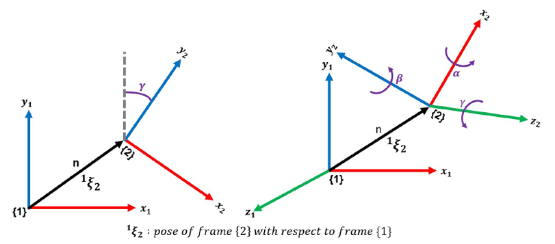
FIGURE 4
Transformations. a) In two dimensions; b) in three dimensions

DENAVIT-HARTENBERG
The Denavit-Hartenberg convention I’m about to explain in this section can be challenging to understand for newcomers. If that’s true in your case, don’t be discouraged. It can take some time to absorb, analyze it thoroughly and to eventually grasp the concept. I would suggest you check some extra material available on the Internet if you want to deepen your understanding of this topic. It’s practically impossible to explain it in reasonable detail in a short article like this, but I’ll do my best.

There’s more than one way to attach frame references to links in a robotic arm. The so-called “Denavit-Hartenberg convention” defines a particular way to do it, and is a popular approach with robotic arms. In this convention, the basic idea is that frame references are attached to joints located at the link ends, such that the rotation component of the transformation must be defined around the “z” axis and is associated with the joint itself. On the other hand, the translation component of the transformation is defined along the “x” axis and is associated with the link length. Figure 3 shows the frame assignment to each joint, including the tip of the end effector in our robotic arm by following this convention.

More concretely, however, in the Denavit-Hartenberg convention, a total of four parameters are used to describe the transformation between two consecutive frames: two rotational parameters (“θ” and “α”) and two linear parameters (“r” and “d”). Figure 5 shows the Denavit-Hartenberg parameters for our robotic arm, along with a succinct description of their meaning. I’ll discuss this in greater depth next.

FIGURE 5
Denavit-Hartenberg parameters for the robotic arm

For a typical robotic arm with rotational joints like ours, the “θ” angles will be the joint rotation angles around their corresponding “z” axes (Figure 6); “r” will be the link lengths along the “x” axes for joints that rotate in a vertical plane (joints 2, 3 and 4 in our robotic arm), and for joint 1, which rotates in the horizontal plane, “r” is zero (there’s no link length in frame {1}’s “x” axis). The “α” angle is the rotation angle of a previous coordinate frame around the “x” axis of the next frame to align the former with the latter.

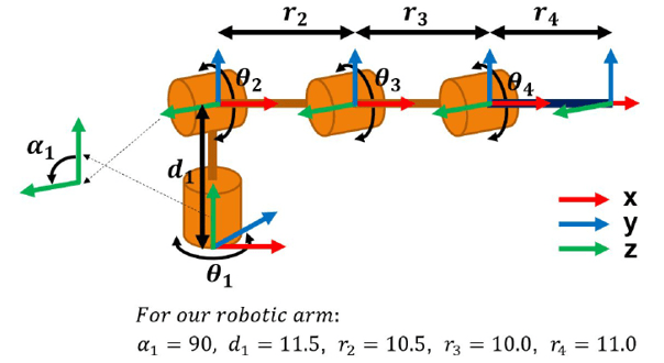
FIGURE 6
Denavit-Hartenberg parameters in relation to the arm structure

For our robotic arm, the transformation from frame {1} to frame {2} will have an “α“ of 90 degrees, because that’s the angle frame {1} must be rotated around the “x” axis of frame {2}, to align frame {1} with frame {2}. In other words, 90 degrees is the angle we must rotate frame {1} to align their “z” axis with the “z” axis of frame {2}. For the transformation between frame {2} and frame {3}, “α“ is zero, because both frames are already aligned (that is, their “z” axes are in the same direction), and the same applies to the next two transformations. All rotations in the convention follow the “right hand rule.”

The “d” parameter indicates the displacement of two consecutive coordinate frames along the “z” axis of the first of the two. The transformation from frame {1} to frame {2} has a “d” parameter equal to the distance between the first and second joints (that is, from the base of the robotic arm to joint 2), because that’s the distance between the two, along the “z” axis direction of frame {1}. However, the displacement of frame {3} from frame {2}, along the “z” axis of frame {2} is zero, and it is the same for subsequent transformations.

Generally, for our type of robotic arm, “α”, “r” and “d” will be constants, but you should change at least “r2”, “r3”, “r4” and “d1” in the MATLAB code to reflect the link lengths of your particular robotic arm structure. The Robotic_Arm_GUI_OpeningFcn() function located in the file “Robotic_Arm_GUI.m” contains all Denavit-Hartenberg constants.

A homogeneous transformation matrix makes it possible to describe mathematically the transformations between coordinate frames. Equation (2) shows how a Denavit-Hartenberg homogeneous transformation matrix is defined by using the four aforementioned parameters (“θ”, “α“, “r” and “d”). In the case of revolute joints, “θ” (the joint angle) is variable and “α“, “r” and “d” are generally constants. Because we have five coordinate frames attached to our robotic arm, we can build four transformation matrices that describe the pose of each subsequent coordinate frame with respect to the previous one, with each one built by using their specific parameters. For instance, to obtain the first homogeneous transformation matrix (transformation from frame {1} to frame {2}), we must use the parameters from row 1 in Figure 5, row 2 for the transformation from frame {2} to frame {3}, and so on.

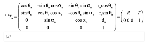
^n-1T_n : transformation from 0_n-1 (frame_n-1) to 0_n (frame_n)
R : rotation component
T : translation component

FORWARD KINEMATICS
Forward kinematics is the task of computing the position of the end effector from a given joint configuration—that is, a set of joint angles. Equation (3) gives us the general forward kinematics formula. To do so, we have to compute the homogeneous transformation matrix that describes the pose of the end effector (frame {5}) relative to the base of the robotic arm (frame {1}) by multiplying all four transformation matrices defined for consecutive coordinate frames, as described by Equation (4) and illustrated in Figure 7.

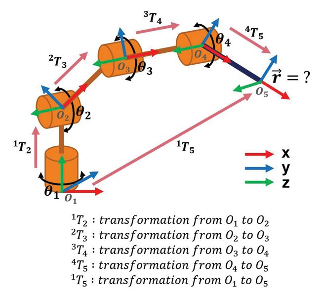
FIGURE 7
Robotic arm forward kinematics

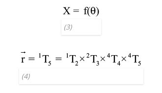
The resulting transformation matrix from frame {1} to frame {5} gives us the position of the tip of the end effector with respect to the body frame; which will generally be the “world” frame or the coordinate frame, in which all required poses for the robotic arm will likely be given—for example, the coordinates of an object the robotic arm must pick up. So, for calculating the forward kinematics given a new set of joint angles, first we calculate the individual transformation matrices using the new “θ” joint angles, then we multiply them in the given sequence to obtain the new end effector position.

In the “Run_Plot_Fwd_Kinematics.m” file, the code line fwd_kin_result = Calc_Fwd_Kinematics(dh_params) calls the function that will compute the forward kinematics. This function (located in the file “Calc_Fwd_Kinematics.m”) will compute the four new transformation matrices and then multiply them to obtain the new end effector’s position.

If we calculate the partial derivatives of Equation (3) with respect to “θ”, we obtain Equation (5), which is called the Jacobian.

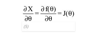
The Jacobian expresses the rate in change of the linear components in “x”, “y” and “z” of the moving tip of the end effector, with respect to the change in joint angles. So, the Jacobian basically tells us what a tiny displacement of the tip of the arm we expect to have in “x”, “y” and “z”, in relation to tiny increments/decrements of the joint angles. This is a particularly useful mathematical intuition that will help us understand the inverse kinematics method I’ll explain next.

INVERSE KINEMATICS
Inverse kinematics, as the name implies, is the inverse process of finding the joint angles that correspond to a given position of the end effector in 3D space. Figure 8 illustrates the concept and Equation (6) gives us the general mathematical formula.

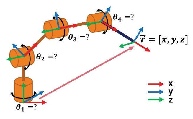
FIGURE 8
Robotic arm inverse kinematics

The “Jacobian Transpose” and the “Jacobian Pseudo-inverse” are two well-known iterative methods for computing the inverse kinematics. Equation (7) shows the general formula for the Jacobian Transpose inverse kinematics method, which resembles Equations (5) and (6).

ΔX: delta of displacement in x , y, z
Δθ: delta of all joint angles

The Jacobian transpose method allows us to compute a tiny increment/decrement in joint angles that corresponds to a given tiny movement of the tip of the end effector in 3D space. Thus, it can be used iteratively to calculate the inverse kinematics necessary to take the end effector to a new position. To do so, we first calculate the Euclidean distance between the start (actual) position and the end (desired) position of the end effector. Then we extract its components in “x”, “y” and “z” and divide them by a factor of, say, 10 or 20. Because the Jacobian is a linear approximation, it will work better over tiny displacements. The vector of those three components will be our delta displacement in position “ΔX” (ΔX = [δ x, δ y, δ z]).

Second, we calculate the Jacobian matrix with the current joint configuration (that is, the set of start “θ” angles that correspond with the start position). Third, we multiply the Jacobian matrix by “ΔX” (and a scaling factor “α”) to obtain a vector “Δθ” (Δθ = [δθ₁, δθ₂, δθ₃, δθ₄]) that gives us the corresponding angle increment/decrement for each joint that will cause the aforementioned “delta” displacement in position of the arm’s tip—which will be the tenth or twentieth of the initial Euclidean distance. Fourth, after modifying the joint angles for a value of “Δθ” (i.e. θ = θ + Δθ), we take these new angles and the resulting intermediate position of the end effector as a start, and repeat the process iteratively, until the Euclidean distance is small enough (say, 10^-3) for us to consider the error negligible for practical purposes.

The Jacobian pseudo-inverse kinematics method is a similar method, in which we use the pseudo-inverse of the Jacobian instead of the transpose. The pseudo-inverse is said to be computationally faster than the transpose, and the procedure and results are almost the same: We compute the Jacobian pseudo-inverse matrix and multiply it by “ΔX” to also obtain “Δθ”, and repeat that iteratively. Equation (8) shows the general formula for the Jacobian pseudo-inverse kinematics, and Equation (9) shows the formula of the Jacobian pseudo-inverse.

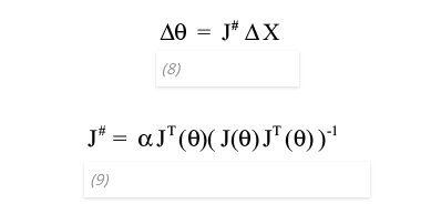
Code lines 572 through 596 from the button_calc_invkin_Callback() function in the “Robotic_Arm_GUI.m” file show the implementation of the Jacobian pseudo-inverse kinematics algorithm. Computing the pseudo-inverse or the transpose of a matrix in MATLAB is as easy as calling the “pinv” or the “transpose” MATLAB functions.

The start pose is the default pose of the robotic arm when the system is initiated. The pose at zero degrees for all joints (Figure 3 and Figure 6) isn’t particularly appealing as a start pose, for both practical and esthetic reasons. Figure 9 shows a more convenient one with a joint configuration q = {0, 90, -90, -90}. This start pose is programmed in the Robotic_Arm_GUI_OpeningFcn() function to be set by default when the GUI is opened. See code lines 114 through 140 in the aforementioned function.

FIGURE 9
Robotic arm start pose

TESTING THE ROBOTIC ARM
I highly recommended that you first test and debug the robotic arm by sending manual commands to the embedded controller. Once that works well, proceed to test it with the MATLAB code. To do so, connect the embedded controller to the companion computer and open the Arduino’s USB port from the Arduino IDE’s Serial Monitor (or another software terminal emulator), to manually send commands to the embedded controller and drive the joint motors. For instance, you can send the command “2$-13&” to select joint 2 and move it to -13 degrees (see Part 1 of this article for the command protocol specification). The embedded controller’s serial command interface also implements additional test commands. For instance, if you type “+” the current selected joint (for example, joint 2) will increase its angle by 10 degrees, and if you type “-” it will decrease it by the same amount.

It is also possible to send multiples of these commands, such as “+++” to increase the angle by 30 degrees, or “—-” to decrease it by 40 degrees and so on. A “c” command will take the current selected joint to the default angle (the start pose). If you want to change the current selected joint, just type the joint number, for example “3” to change to joint 3. If you want to change the current selected joint and at the same time move it, you can type, for example, “4++”. That will change the current joint to four, and then increase its angle by 20 degrees.

Once the robotic arm works well with manual commands, you can test it with the MATLAB code by running the “Robotic_Arm_GUI.m” file to open the GUI. Be sure to have the Arduino board’s USB cable connected to the companion computer and the assigned virtual serial port name changed in the Robotic_Arm_GUI_OpeningFcn() function before attempting to run the MATLAB code.

Meanwhile, the embedded controller outputs debugging messages serially via pin 6 in the Arduino board (check the circuit diagram from Part 1 of this article). You can connect a USB to UART interface’s serial input pin to pin 6 of the Arduino to receive debug messages in a software terminal emulator, and check the operation of the embedded controller at all times.

CONCLUSIONS AND UPGRADES
The arm structure and servo motors I used for the prototype don’t have a particularly stable or accurate performance. Nevertheless, the robotic arm performs pretty well for its stated purpose, which is to exemplify key concepts, such as PID control, controller/computer interfacing, forward/inverse kinematics and their implementation in code.

Some improvements I have in mind for this project are the following:

First, I would like to try to make the robotic arm draw on a surface. For that, the robotic arm would have drawing paths stored in arrays, as sequences of goal coordinates that it must follow one by one, until the last one is reached.

Second, I would like to try adding computer vision to the robotic arm, to be able to recognize objects, extract their location and automatically fetch and move them to other places.

Third, I would like to add two more degrees of freedom, optionally using at least one prismatic joint. It would be interesting as well to gradually replace the servo motors with DC motors, each one with its corresponding PID control loops. I could also try to build my own “smart servo motors,” by embedding to each DC motor its own H-bridge driver and microcontroller for the PID control loop.

Finally, I would like to convert the MATLAB companion computer code to the Python programming language, which is open source and free, and it’s preferred in some educational settings. By having a Python version, more people would potentially benefit from the work presented in this project. Converting the MATLAB code to Python—or any other language for that matter, is a good exercise I can recommend to anyone willing to delve deep into the algorithms described in this project. To convert the code correctly, you must reach a reasonable understanding level of the involved algorithms. And, while doing so, you’ll gain a reasonable understanding of the source and target languages. 

For detailed article references and additional resources go to:
www.circuitcellar.com/article-materials
References [1] through [6] as marked in the article can be found there.

最后预告一下今天下午的直播课程 - 入门PCB设计的正确姿势（2）：电子产品的系统构成及关键元器件的选用。想学习PCB设计和FPGA编程的同学可以扫描下面的二维码，经我们的工作人员审核以后可以加入我们的课程交流群。

课程详情，请点击左下角的“阅读原文”。