这是选自国外杂志“CircuitCellar”上的一篇技术文章,介绍如何用Matlab和Arduino制作一个4自由度的机械臂。这是文章的第一部分,第二部分会在后续的文章中再做介绍。
Using MATLAB and Arduino
When it comes to building your own robotics systems, the future is truly now, thanks to inexpensive hardware and software tools available today. In this project article, Raul explains how he built a robotic arm with four degrees of freedom (4-DOF) and revolute joints. For anyone interested in introductory robotics, this low-cost hardware and software platform lets you get up and running.
In this article, I discuss my project that implements a robotic arm with four degrees of freedom (4 DOF) and revolute joints (often denoted as RRRR), for the purpose of studying and experimenting with forward/inverse kinematics and PID control basics applied to robotic arms. It uses a DC motor with a bi-phase encoder for the first joint at the base of the arm, and digital servo motors for the remaining three joints—including one additional servo motor for the end effector. The angular position of the DC motor is controlled with a PID control loop. The remaining servo motors are controlled with open-loop control signals, because servo motors already have closed-loop controls implemented in hardware.
The robotic arm has an embedded controller that runs the PID algorithm for controlling the angle of the DC motor, and also controls the servo motors. In addition, for changing joint angles, it implements a communication interface to receive commands through the serial port.
The forward and inverse kinematics algorithms are implemented using Mathwork’s MATLAB programming language. They are run in a companion computer, which interfaces to the embedded controller by using the serial communications command interface. The MATLAB code also implements a Graphical User Interface (GUI), from which the user can control the robotic arm and run the forward and inverse kinematics algorithms. A 3D simulation/visualization of the robotic arm is displayed in the GUI in real time.
The aim of this project is to provide anyone interested in introductory robotics with a low-cost hardware and software platform that allows easy experimentation with forward and inverse kinematics algorithms, PID control and controller/computer interfacing.
Figure 1 is a block diagram showing the main components of the robotic arm. The embedded controller determines the pose of the robotic arm by commanding each of the four joint motors to the desired angles. It implements a serial command interface with a very simple ASCII string protocol for receiving target angles from the companion computer. It also implements a PID control loop for controlling the rotation angle of the DC motor at joint 1.
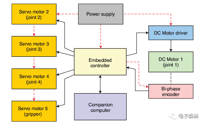
FIGURE 1 Robotic arm block diagram
To do so, it reads the current motor position from the bi-phase encoder attached to the DC motor, and computes the required PID output signal to drive the motor to the target angle. The servo motors are handled much more easily by using only an open-loop control scheme. As noted earlier, forward and inverse kinematics algorithms are written in MATLAB and run in the companion computer. Both algorithms return a set of angles for each of the four joints, which are then sent to the embedded controller via the serial communications interface. For the companion computer, I’m using a regular personal computer with Windows 10 operating system installed.
ELECTRONICS HARDWARE
The circuit schematic for the robotic arm is shown in Figure 2. For the embedded controller, I’m using an Arduino UNO board, which is very intuitive for beginners and makes it easy to interface a wide variety of sensors and actuators. With it, there is no need to worry about low- or mid-level drivers and libraries for performing basic functions—such as driving a motor, doing serial communications or managing external interrupts.
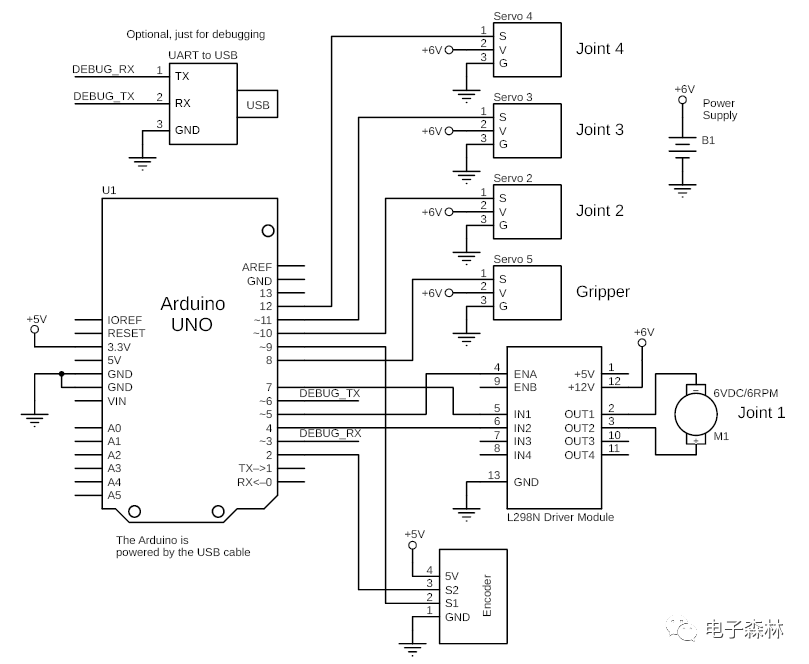
FIGURE 2 Circuit schematic for the robotic arm
Case in point: I’m using the Arduino microcontroller’s (MCU) external interrupts to promptly detect the ticks generated by the encoder attached to the DC motor in joint 1. Fast tick detection and counting is very important for the PID control algorithm. Besides, the Arduino UNO board is low-cost and easily programmed just by using an ordinary USB cable. The cable also can be used to interface the board with the MATLAB code running in the companion computer, by opening it as a virtual serial port.
I have chosen a DC motor for the first joint at the base of the robotic arm specifically to illustrate angular position embedded PID control. By including it as a hardware and software implementation example, it serves as a means of studying the concept; hopefully easy to understand for those new to this concept. And, by including it as a hardware and software implementation example, it is easy to understand for those new to this concept. For the other joints, I chose servo motors to keep the rest of the code simpler. Arguably, all servo motors can be replaced by DC motors by just duplicating the hardware and PID control code that already works for joint 1. I would recommend beginning by replacing just one servo motor and once it works well, proceed with the next, and so on. The kinematics code in the companion computer should work just fine with the replaced motors, because it is totally independent of the hardware implementation of the robotic arm.
The DC motor at joint 1 is a generic JGY370 DC motor [1] that spins at 6 RPM when powered with 6 VDC. It has a torque of 14 kg- cm, which is more than enough to rotate the whole robotic arm horizontally, and it comes with an attached generic bi-phase encoder. The motor is driven by a STMicroelectronics L298, 2-channel H-bridge Driver Module. If you want to try DC motors with PID controls in the rest of the joints, first make sure to have motors with the required torque for each joint. This is important because the torque necessary to rotate weights in a vertical plane generally must be greater than that for rotating them in a horizontal plane.
The bi-phase encoder attached to DC Motor 1 has a resolution of 6,300 ticks per revolution (that is, it provides 6,300 pulses every full rotation). Theoretically, this gives a resolution of 17.5 ticks per degree, which is more than enough for our robotic arm. If you use an encoder with a different resolution, don’t forget to change the related constant ENC_TICKS_PER_REV in the Arduino code, otherwise you won’t get the exact commanded angle. If you don’t know the resolution of your encoder, you can measure it by commanding the motor a certain amount of degrees (say, 360 degrees or more), print the ticks in the Arduino IDE’s serial monitor, and then use the “rule of three” to obtain the number of ticks per revolution for your encoder.
MORE ON THE JOINTS
For joints 2 to 4 and the end effector or “gripper,” I’m using JX Servo PDI-6221MG 20 kg-cm digital servo motors [2]. Digital servo motors have smaller dead bandwidth compared to typical analog ones. This helps to reduce vibration when the links are horizontally extended and the servo motors are holding against downward rotational forces generated by the arm’s weight and load. I’m powering the servos with 6 VDC, which is the maximum allowed power voltage for these servo motors, to obtain their maximum torque performance. Lower torque servo motors can be used for joints 3, 4 and the gripper, but I’m using the same servos on all joints because that’s what I had at hand.
The power supply must be able to provide the required current for all motors. I have connected my bench power supply adjusted to 6 VDC, which can provide up to 5 A. The Arduino UNO board is powered from the USB cable connected to the companion computer, which also powers the bi-phase encoder.
Finally, for the companion computer, I’m using a regular laptop with MATLAB R2015a installed on it. Any personal computer can be used, provided that it has the minimum recommended specifications to run MATLAB software.
For the mechanical frame, I picked an off-the-shelf aluminum robotic arm kit [3] to ease the mechanical implementation and concentrate all efforts on the electronics and code parts of the system. This is a generic kit very popular among beginners. It’s really easy to put together in a couple of hours, and has all parts for a complete robotic arm structure. I built a wood base to which I attached the robot arm with screws, to have a more solid stand. Figure 3 shows the robotic arm assembled with all its parts.
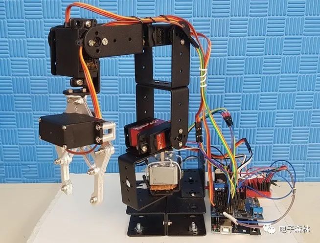
FIGURE 3
Fully assembled robotic arm
It is important to have motors with the correct torque specifications for each one of the joints, otherwise they would not be able to counter the rotational torque in each joint due to the weight of each link and their corresponding loads. There are free online apps to calculate torque for robotic arm joints [4]. You need to provide inputs, such as the configuration of the robotic arm (how many degrees of freedom it has), link lengths, link weights, loads and so on.
They’ll compute the necessary torque for each joint for the worst-case scenario—lifting weights at 90 degrees from the vertical—that is, with the links horizontally fully extended. If you don’t want to deal with the calculations, it is possible to set the torques by trial and error, testing the motors with their links at 90 degrees from the vertical and with full loads, and oversizing them a bit just to be sure they will cope well with the loads. There’s a fifth servo motor for the end effector (the gripper). However, it doesn’t get counted as a degree of freedom for the robotic arm, so I will ignore it when talking about kinematics.
EMBEDDED CONTROLLER
The embedded controller firmware is written in C/C++ for the Arduino platform. I’m using the “Servo” and “Serial” libraries included by default in the Arduino platform to control the servo motors and to do the serial communications. Although a PID control library for Arduino is also available, I chose to write my own PID control routine. I did this because I wanted to show how to implement it in code “by hand,” for those who are new to it. Besides, it is more portable, in case you want to try PID in another MCU platform. The embedded controller also implements a low-pass filter for filtering angle readings, and a serial command parser, which will be discussed in more detail later.
The embedded controller receives angle commands for each of the joints from the companion computer through the serial port, in a very simple protocol format devised for that purpose. Figure 4 shows an example of angle data packed for DC Motor 1 in the aforementioned protocol. The angle value is packed along with some delimitation symbols. These delimitation symbols help the embedded controller to discriminate the angle data in the received frames. Figure 5 is an example of angle data packed for all four joints. The embedded controller detects the delimitation symbols when parsing the serial data, and can easily know which characters correspond to angles and for what joints. When an Arduino board is connected to a computer, it is recognized by the operating system as a “virtual serial port,” so to send data from MATLAB, we just have to open the virtual serial port in code and send the data in ASCII format.
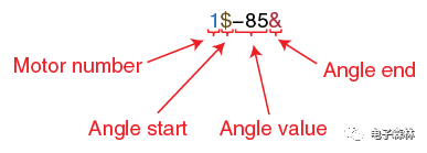
FIGURE 5 Packed angle data for all four motors
This serial interface also becomes handy when debugging the basic angle control of the joints. We can manually open the virtual serial port in Arduino IDE’s serial monitor, or by using any other terminal emulator software (such as Putty or Tera Term), and send angle command data frames by typing them in the format shown in Figure 4 and Figure 5. In fact, it is highly recommended to test and debug the hardware in this way before connecting the robotic arm to the companion computer. This allows the correct rotation of every joint to be checked, before interfacing the arm with the MATLAB code.
PID CONTROL AND FILTERING
A PID (proportional–integral–derivative) controller is a control-loop mechanism widely used in many control systems, including robotics [5]. This controller calculates an error value as the difference between a desired setpoint (in our case, some desired angle for joint 1) and the actual measured process variable (the actual measured joint 1 angle). It then uses this error to calculate an output signal composed of the sum of three terms: The proportional, integral and derivative (P, I and D, hence the given name). The output signal then is applied to the actuator as a correction signal to drive the error to zero—or more realistically, within a given error tolerance that the system can cope with. The PID control uses a feedback loop to measure the error iteratively, calculate and apply the output signal to the actuator. This closed-loop configuration is what makes this type of control very responsive, accurate and independent of external system parameters. Figure 6 is a graphical representation of the PID controller used with the DC motor at joint 1.
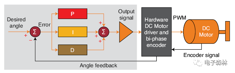
FIGURE 6 PID control loop for DC Motor 1
Every time a sensor is used to read some variable in the environment (such as position or velocity), a certain amount of noise (typically random) will always be present in that reading. This noise is due to some factors such as the error tolerance of the sensor itself, including external perturbations in the environment and magnetic interference. Generally, this sensor noise will be a high-frequency signal in comparison with the frequency of the signal or data of interest. It tends to mess with the performance of the PID controller, because the controller will try to react to the high-frequency oscillating noise, instead of trying to correct for the signal of interest. That, in turn, will cause oscillations in the system and also make it more difficult to tune the PID constants.
Some systems are more sensitive than others to noise. It depends on their specific characteristics. For systems that are very sensitive to noise, a filter helps to reduce the amount of noise present in the sensor data, thus improving the performance of the PID controller. I implemented a low-pass, moving-average filter in the embedded controller [6] to smooth the high frequency noise and help the PID algorithm to drive the motor more easily to the desired angle. This kind of filter is generally the easiest way to implement sensor noise filtering in an MCU. It is very popular and works well with many types of sensors.
A PID control system has three tuning constants, Kp, Ki and Kd, which control the gain or contribution of each of the three terms (proportional, integral and derivative) to the output signal sum. By appropriately setting these three constants, we make the system’s response to error as fast and stable as possible. The PID constants I provide in the Arduino code work well with my setup, but may not work as well with yours if you deviate somehow from the proposed hardware.
For example, you might have differences in motor velocity, encoder resolution, joint friction and mass of your robotic arm structure. In that case you may need to re-tune the three constants from zero. Depending on your previous experience with PID, there are some tuning methods you can use, the easiest of which—iterative trial and error—is generally recommended for beginners. (I use it all the time.) There are many resources on the Internet for learning how to use it, in case you aren’t familiar with it.
MATLAB GUI BASICS
Figure 7 shows the GUI that I made for the robotic arm, using MATLAB’s GUI Development Environment. In the following paragraphs I’ll explain some basic concepts about how a GUI works in MATLAB, and how it interfaces with the application code to perform the desired tasks. I won’t explain how to build the GUI from scratch, but there are some online tutorials if you want to learn how to do it.
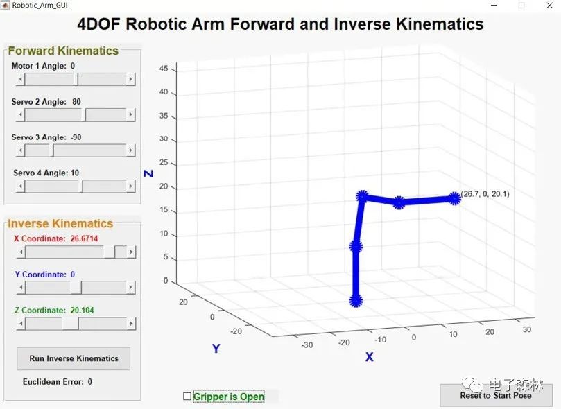
FIGURE 7 MATLAB Graphical User Interface
In a MATLAB GUI, the components used to input data—such as buttons, sliders and check boxes—are generally attached to callback functions in code. So, any time you interact with one of these components, for example, by clicking a button or moving a slider, its corresponding callback function is called. This means that these callback functions must contain all the code you want to run in response to interactions with these controls.
The provided MATLAB code file “Robotic_Arm_GUI.m” contains all GUI callback functions. For instance, when the “Motor 1 Angle” slider is moved (Figure 7), the slider_motor1_angle_Callback() function is called. Inside it, the following tasks are performed: get the new angle value for Motor 1 (set by the moved slider); compute the forward kinematics and plot the new resulting pose; update the “Motor 1 Angle” text label in the GUI with the new angle value; update also the resulting X, Y and Z coordinates of the end effector (the tip of the arm) in the corresponding coordinate sliders and text labels; and finally, send the new angles through the serial port to the embedded controller, for moving the robotic arm to the new pose. The same applies for the other angle sliders.
Also, when the ”X Coordinate” slider is moved, the callback function slider_coordx_Callback() is called to perform the following tasks: it reads the values from all three coordinate text labels (X, Y and Z), and stores them in an array (these are the target coordinates to move the arm by running inverse kinematics); then, it updates the changed coordinate value in the X-coordinate’s text label. When the “Run Inverse Kinematics” button is pushed, the button_calc_invkin_Callback() function is called. It will read the previously stored target coordinates and run the inverse kinematics algorithm to compute new angles for each one of the joints, plot the new pose in the GUI, and then send the angles to the embedded controller. The same applies for the Y and Z coordinates.
When the “Reset to Start Pose” button is pushed, the button_reset_Callback() function is called. It resets all angles and coordinates to their initial values, updates the robotic arm’s pose in the GUI and sends these initial angles to the embedded controller to reset also the real robotic arm.
The MATLAB GUI code also has an “opening function” called Robotic_Arm_GUI_OpeningFcn() that runs once, when the GUI window is created. It also has a “closing function” called figure_gui_CloseRequestFcn() that runs every time the GUI window is closed. In the opening function, the following tasks are performed: open the virtual serial port associated with the Arduino UNO—don’t forget to change this for your own before running the MATLAB code; set all initial values for the robotic arm (for example, angles, coordinates, link parameters); and plot the robotic arm’s initial pose in the GUI. In the closing function, the most important task performed is closing the serial communications port, because if left open, the application will throw an error the next time it runs and tries to access it.
MATLAB COMMS AND PLOTTING
To send data from the companion computer to the embedded controller via the virtual serial port (that is, the Arduino UNO’s USB cable connected to the computer), the serial port must be properly configured and open. This is easy to do with the available serial port functions in MATLAB. (See the aforementioned “opening function” in the code.) Sometimes, when debugging the serial communications, the MATLAB code will crash without properly closing the serial port. If this happens, you can type “instrreset” in the MATLAB Command Window to close the serial port that was left open, before running the code again.
Once the serial port is open, sending data to the embedded controller is just as easy as calling MATLAB’s “fprintf” function. For instance, fprintf(serial_port, strcat(‘2$’, num2str(round(angle2)), ‘&’)) sends the angle data frame for servo motor 2. Finally, in the “closing function,” the serial port will be closed before finishing the MATLAB application.
The Run_Plot_Fwd_Kinematics(theta1, theta2, theta3, theta4) function (contained in the “Run_Plot_Fwd_Kinematics.m” file) is in charge of plotting the robotic arm pose in the GUI. This function receives as parameters the new joint angles of the robotic arm, and calls inside the Calc_Fwd_Kinematics(dh_params) function. This function calculates the forward kinematics and returns a matrix containing the X, Y and Z coordinates of the ends of each one of the robotic arm’s links. These coordinates will then be used by the caller function to plot the arm’s graph in the GUI.
For simplicity, I’m using a simple “wire graph” plot of the robotic arm links (no fancy 3D stuff!) to keep the code readable for those who are new to MATLAB programming. The “plot3d” function used for this purpose basically takes as arguments three vectors of the X, Y and Z coordinates (among other arguments, such as line width and color), and lets you draw lines and dots in three dimensions. I’m passing as arguments the first three rows of the matrix returned by the forward kinematics calculation, which contain the X, Y and Z coordinates of both ends of every link in the robotic arm to plot the arm’s pose. Every time the pose changes, the forward kinematics is calculated again to obtain the new coordinates, and the plot is refreshed in the GUI.
WHAT’S NEXT?
Figure 8 shows the complete system, comprising the robotic arm, the embedded controller and the companion computer. The project files for this project are available on Circuit Cellar’s article code and files download webpage. In those project files, there are detailed instructions for setting up and running the system.
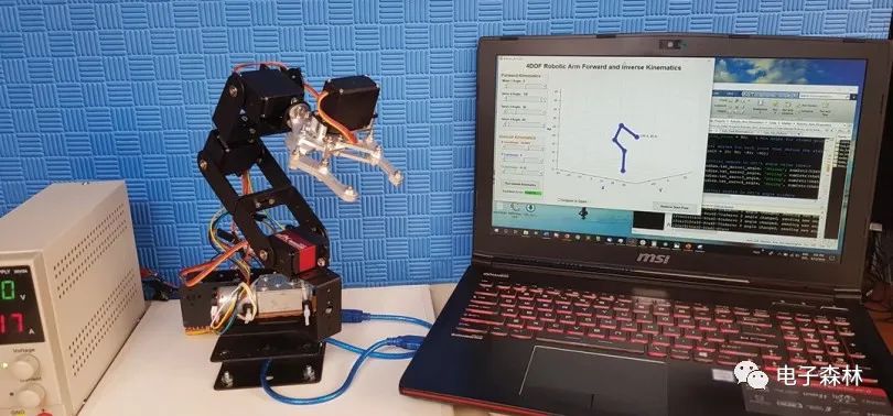
FIGURE 8 Robotic arm, embedded controller and companion computer
In Part 2 of this article series, I’ll be discussing topics more related to the mathematical foundations of robotics, such as configuration spaces, robot pose representation in three dimensions, homogeneous transformations, Denavit-Hartenberg parameters, direct kinematics and inverse kinematics with the pseudo-inverse Jacobian. I’ll also talk a bit about testing, my conclusions and future improvements. Part 2 is scheduled to appear in the February 2020 issue (Circuit Cellar 355). Stay tuned!
For detailed article references and additional resources go to:
www.circuitcellar.com/article-materials
References [1] through [6] as marked in the article can be found there.
